

1 Représentations graphiques de fonctions
Inclure le module pst-plot (\usepackage{pst-plot}).
Définitions supplémentaires utilisées dans certaines figures
:
\newcommand{\repere}{
  \psset{ticksize=.7pt,linewidth=.7\pslinewidth,labelsep=2.5pt}
  \pstGeonode[PosAngle=-135]{O}
  \pcline{->}(0,0)(1,0)\rput(0.5,-0.4){$\vec i$}
  \pcline{->}(0,0)(0,1)\rput(-0.5,0.5){$\vec j$}}

\newcommand{\markpoint}[4][]{\pstGeonode[#1](#2,#3){#4}
  \psline[linestyle=dashed](0,#3)(#2,#3)(#2,0)}
\begin{toimage}
\psset{unit=7mm,labels=none}
\end{toimage}
\begin{figure*}[h]
\centering
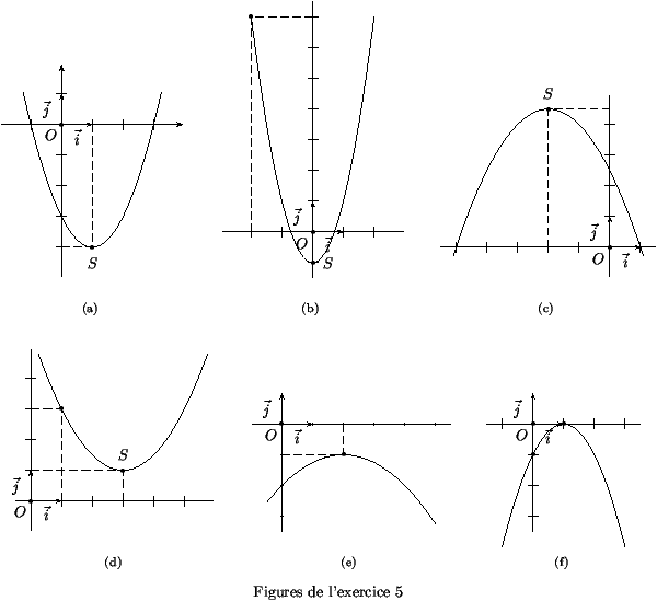
\subfigure[]{\begin{pspicture}(-2,-5)(4,2)
\psaxes{->}(0,0)(-1.95,-4.95)(3.95,1.95)
\repere
\def\F{x 1 sub 2 exp 4 sub}
\psplot{-1.25}{3.25}{\F}
% \pstGeonode[PosAngle=-90](1,-4){S}
% \psline[linestyle=dashed](0,-4)(1,-4)(1,0)
\markpoint[PosAngle=-90]{1}{-4}{S}
\end{pspicture}}
\qquad
\subfigure[]{\begin{pspicture}(-3,-1.5)(3,7.5)
\psaxes{-}(0,0)(-2.95,-1.5)(2.95,7.5)
\repere
\def\F{x 2 exp 2 mul 1 sub}
\psplot{-2}{2}{\F}
\pstGeonode(0,-1){S}
\markpoint[PosAngle=90,PointName=none]{-2}{7}{I}
\end{pspicture}}
\qquad
\subfigure[]{\begin{pspicture}(-5.5,-1)(1.5,5)
\psaxes{-}(0,0)(-5.5,-0.95)(1.5,4.95)
\repere
\def\F{x 2 add 2 exp -1 2 div mul 9 2 div add}
\psplot{-5.1}{1.1}{\F}
\markpoint[PosAngle=90]{-2}{4.5}{S}
\end{pspicture}}
\subfigure[]{\begin{pspicture}(-.5,-1)(6,5)
\psaxes{-}(0,0)(-.5,-.95)(5.95,4.95)
\repere
\def\F{x 2 exp 2 div x 3 mul sub 11 2 div add}
\psplot{.25}{5.75}{\F}
\markpoint[PosAngle=90]{3}{1}{S}
\markpoint[PointName=none]{1}{3}{I}
\end{pspicture}}
\qquad
\subfigure[]{\begin{pspicture}(-1,-3.5)(5.5,.5)
\repere
\psaxes{-}(0,0)(-.95,-3.5)(5.5,.5)
\def\F{x 2 exp -1 4 div mul x add 2 sub}
\psplot{-.5}{5}{\F}
\markpoint[PointName=none]{2}{-1}{S}
\end{pspicture}}
\qquad
\subfigure[]{\begin{pspicture}(-1.5,-3.5)(3.5,.5)
\psaxes{-}(0,0)(-1.5,-3.5)(3.5,.5)
\repere
\def\F{x 2 mul x 2 exp sub 1 sub}
\psplot{-1}{3}{\F}
\pstGeonode[PointName=none](1,0){S}
\pstGeonode[PointName=none](0,-1){S}
\end{pspicture}}
\label{figs}
\centerline{Figures de l'exercice 5}
\end{figure*}
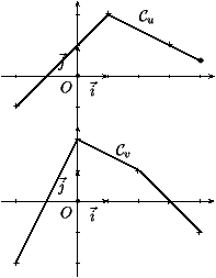 |
\begin{pspicture}(-2.5,-1.5)(4.5,2.5)
  { \repere
    \psaxes{->}(0,0)(-2.45,-1.75)(4.45,2.45)}
  \psset{PointName=none,PointSymbol=+}
  \pstGeonode(-2,-1){A}\pstGeonode(1,2){B}\pstGeonode(3,1){C}
  \pstGeonode[PointSymbol=*](4,.5){D}
  \psline(A)(B)(C)(D)
  \put(2,1.8){$\mathcal{C}_u$}
\end{pspicture}

\begin{pspicture}(-2.5,-2.5)(4.5,2.5)
  {\repere
    \psaxes{->}(0,0)(-2.45,-2.45)(4.45,2.45)}
  \psset{dotstyle=+}
  \psdots(-2,-2)(0,2)(2,1)(3,0)(4,-1)
  \psline(-2,-2)(0,2)(2,1)(3,0)(4,-1)
  \put(1.25,1.5){$\mathcal{C}_v$}
\end{pspicture}
|
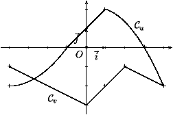 |
\begin{pspicture}(-4.5,-3.5)(4.5,2.5)
  {\repere
    \psaxes{->}(0,0)(-4.45,-3.45)(4.45,2.45)}
  \psset{dotstyle=+}
  \psdots(-4,-1)(0,-3)(1,-2)(2,-1)(4,-2)
  \psline(-4,-1)(0,-3)(1,-2)(2,-1)(4,-2)

  \psdots(-4,-2)(-1,0)(1,2)(3,0)(4,-2)
  \def\Fa{2 9 div x 1 add mul x 7 add mul}
  \def\Fc{0 1 sub 3 div x 3 sub mul x 2 add mul}
  \psplot{-4}{-1}{\Fa}
  \psplot{1}{4}{\Fc}
  \psline(-1,0)(1,2)
  \put(-2,-2.8){$\mathcal{C}_v$}
  \put(2.5,1){$\mathcal{C}_u$}
\end{pspicture}
|
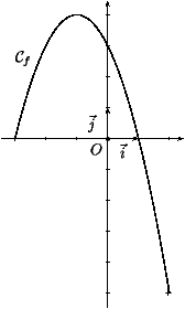 |
\begin{pspicture}(-3.5,-5.5)(2.5,4.5)
  {\repere
    \psaxes{->}(0,0)(-3.45,-5.45)(2.45,4.45)}
  \psset{dotstyle=+}
  \psdots(-3,0)(2,-5)
  \def\F{0 x 1 sub sub x 3 add mul}
  \psplot{-3}{2}{\F}
  \put(-3,2.5){$\mathcal{C}_f$}
\end{pspicture}
|
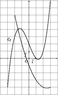 |
\psset{unit=0.7cm}\begin{pspicture}(-4,-5)(4.5,8)
\psset{gridcolor=gray,gridlabels=0pt,subgriddiv=0}\psgrid(-4,-5)(4,8)
  {\repere
    \psaxes{->}(0,0)(-4,-5)(4,8)}
  \psset{dotstyle=+}
  \def\F{x 3 exp 1 2 div mul x 5 2 div mul sub 2 add}
  \def\G{x 2 exp 1 2 div mul x 5 2 div mul sub 1 sub}
  \psplot{-3}{3}{\F}
  \psplot{-2}{3}{\G}
  \put(-3,2.5){$\mathcal{C}_f$}
\end{pspicture}
|
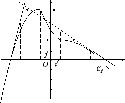 |
\psset{unit=5mm,labels=none}
\begin{pspicture}(-5,-4)(7.5,6)
\renewcommand{\repere}{
  \psset{ticksize=.7pt,linewidth=.7\pslinewidth,labelsep=2.5pt}
  \pstGeonode[PosAngle=-135]{O}
  \pcline{->}(0,0)(1,0)\rput(0.5,-0.4){$\vec \imath$}
  \pcline{->}(0,0)(0,1)\rput(-0.5,0.5){$\vec \jmath$}}

\renewcommand{\markpoint}[4][]{\pstGeonode[#1](#2,#3){#4}
  \psline[linestyle=dashed](0,#3)(#2,#3)(#2,0)}
\newcommand{\hor}[2]{\rput(#1,#2){\pcline{<->}(-1.5,0)(1.5,0)}}

\repere
\psaxes{->}(0,0)(-4.95,-3.95)(7.45,5.95)
\def\f{x 4 add -2 3 div x mul 1 add mul}
\def\g{1 2 div x 2 exp mul -3 2 div x mul add 3 add}
\def\h{-1 8 div x 5 sub x 3 add mul mul}
\psplot{-5}{-1}{\f}
\psplot{-1}{1}{\g}
\psplot{1}{6}{\h}

\pcline[nodesepA=-1,nodesepB=-2](-4,0)(-3,4)
\pcline[nodesepA=-5,nodesepB=-3](1,3)(4,1)

\psset{PointSymbol=none}
\markpoint{-3}{3}{a}\markpoint{-3}{4}{b}
\markpoint{1}{3}{c}\markpoint{4}{1}{d}
\markpoint{-1}{5}{e}

\hor{-1}{5} \hor{1}{2}
\rput(5,-1){${\cal C}_f$}
\end{pspicture}
|
 |
\psset{unit=1cm}
\begin{pspicture}(-2.5,-1)(5,4)
  \psaxes[ticks=none,linewidth=.7\pslinewidth,labels=none]{->}%
  (0,0)(-1.55,-.95)(4.95,3.95)
  \pstGeonode[PosAngle=-135]{O}

  \pstGeonode(0,3){L}
  \pscurve(-1,4)(L)(4,1)
  \psset{linestyle=dashed}
  \pcline(-1,3.45)(3,3.45)\aput(1){$f(x_2)$}
  \pcline(-1,2.65)(3,2.65)\aput(1){$f(x_1)$}
  \pcline(-.5,0)(-.5,4)\lput(-.15){$x_2$}
  \lput(-.25){\psline[linestyle=solid]{->}(-.2,0)(.2,0)}
  \pcline(.5,0)(.5,4)\lput(-.15){$x_1$}
  \lput(-.25){\psline[linestyle=solid]{<-}(-.2,0)(.2,0)}
\end{pspicture}
|
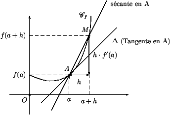 |
\psset{unit=1cm}
\begin{pspicture}(-.5,-1)(6,5)
  \psaxes[ticks=none,linewidth=.7\pslinewidth,labels=none]{->}%
  (0,0)(-1,-1)(5,4)
  \pstGeonode[PosAngle=-135]{O}

  \pstGeonode[PointSymbol=none](0,1){fa}
  \pstGeonode[PosAngle=110](2,1){A}
  \pstGeonode[PosAngle=120](3,3){M}
  \psset{PointSymbol=none}
  \pstGeonode(3.1,4){Cf}
  \pstGeonode(4,0){x}
  \pstProjection{O}{fa}{M}{fah}
  \pstProjection{O}{x}{A}{a}
  \pstProjection{O}{x}{M}{ah}
  \pstProjection{M}{ah}{A}{h}

  \pscurve(fa)(1,.7)(A)(M)(Cf)
  \uput[l](Cf){$\mathscr{C}_f$}
  \pcline[nodesep=-2](A)(M)\bput(1){sécante en A}
  \pcline[nodesep=-2](A)(3,2)\bput(.9){$\Delta$ (Tangente en A)}

  \pcline{<->}(A)(h)\Bput{$h$}
  \pcline{<->}(h)(M)\Bput{$h\cdot f'(a)$}

  \psset{linestyle=dashed}
  \pcline(fa)(A)\uput[l](fa){$f(a)$}
  \pcline(a)(A)\uput[d](a){$a$}
  \pcline(fah)(M)\uput[l](fah){$f(a+h)$}
  \pcline(ah)(M)\uput[d](ah){$a+h$}
\end{pspicture}
|